Bayesian BLP: Structural Demand Estimation on Aggregate Market Shares#
import warnings

import arviz as az
import matplotlib.pyplot as plt
import numpy as np
import pymc as pm
import seaborn as sns
from scipy.stats import norm, qmc

from pymc_marketing.customer_choice import (
    BayesianBLP,
    generate_blp_panel,
    taste_profiles,
)

warnings.filterwarnings("ignore")
az.style.use("arviz-darkgrid")
plt.rcParams["figure.figsize"] = [12, 5]
plt.rcParams["figure.dpi"] = 100
%config InlineBackend.figure_format = 'retina'
The aggregate-data problem#
You have weekly market-share data for a category. You want to know: if I raise the price of product A by 10%, how much share moves to product B versus the outside good? Standard regression on aggregate shares conflates two quantities: the average consumer’s price sensitivity, and the distribution of price sensitivity across consumers. Conflate them and the same 10% hike predicts the wrong substitution pattern in every market that has a different mix of price-sensitive and price-insensitive buyers.
A short example. Market A has 40% share for sugary cereal at average income $30k. Market B has 60% share at average income $50k. A naïve read says higher income drives sugary cereal sales. Within each market the relationship may reverse. The market is a confounder; aggregation hides which way the within-market effect runs. This is the ecological fallacy.
What BLP does#
BLP estimates the distribution of consumer preferences most consistent with the observed aggregate shares. The estimator integrates over latent taste types and asks the Bayesian question: which preference distribution, propagated through a discrete-choice utility model, reproduces what we see in the data? With the distribution in hand, counterfactual prices feed through the same mechanism and give substitution patterns that respect both the average effect and the heterogeneity.
# --- Generate Halton draws ---
sampler_halton = qmc.Halton(d=3, scramble=True)
u = sampler_halton.random(100)

# Avoid infinities in inverse CDF
eps = np.finfo(np.float64).tiny
u = np.clip(u, eps, 1.0 - eps)

# Transform to Gaussian
z = norm.ppf(u)

# IID uniform for comparison
rand = np.random.rand(100, 3)
Halton draws#
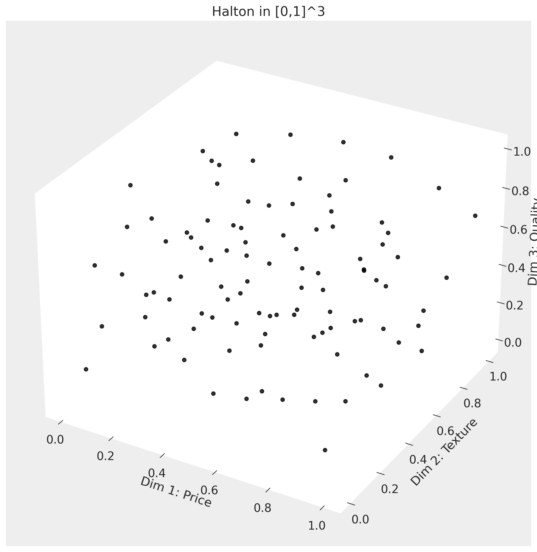
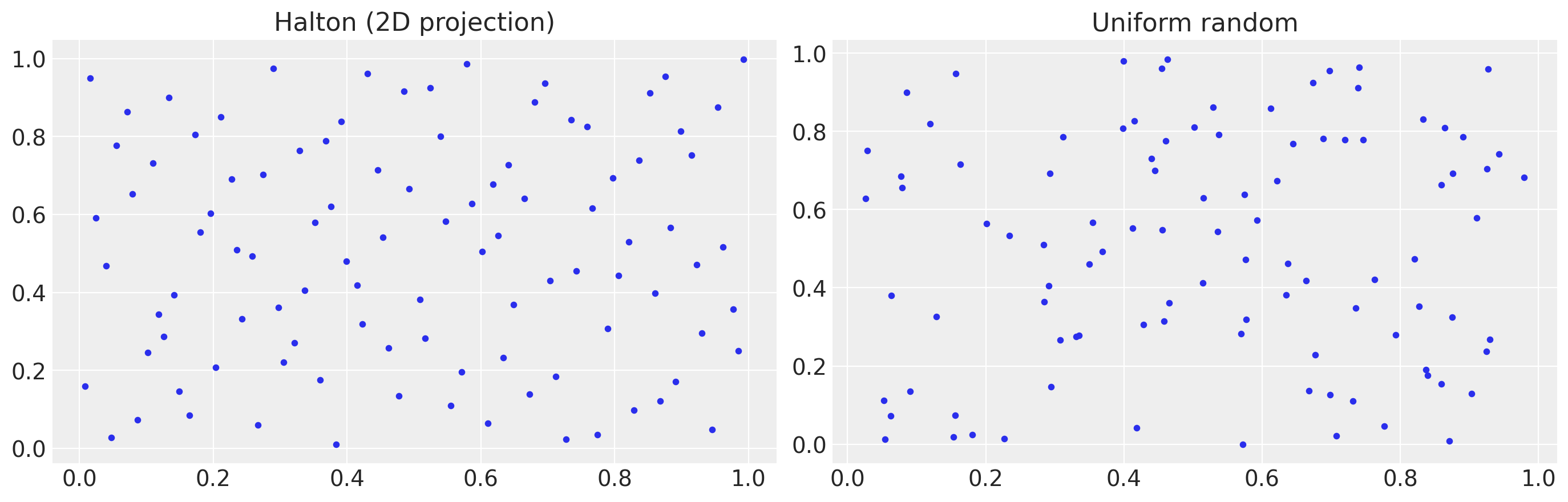
The integral over consumer taste types has no closed form, so we approximate it with a fixed grid of draws. Owen-scrambled Halton draws fill a D-dimensional cube more evenly than the same number of pseudo-random draws (figure below), which means fewer draws for a given accuracy. We treat these draws as data: the model sees the same Halton points on every iteration and learns which taste types are most consistent with the observed shares.
fig = plt.figure(figsize=(20, 8))

# ========== 3. Comparison with random ==========
ax4 = fig.add_subplot(231)
ax4.scatter(u[:, 0], u[:, 1], s=10)
ax4.set_title("Halton (2D projection)")

ax5 = fig.add_subplot(232)
ax5.scatter(rand[:, 0], rand[:, 1], s=10)
ax5.set_title("Uniform random");
The Halton grid feeds the share integral the model evaluates at every draw of the parameters:
The mean utility and the consumer-level deviation are
where \(c_{jmd}\) is the value of the \(d\)-th random_coef_on covariate for product \(j\) in market \(m\) (price, or any product characteristic the user passes). \(\delta_{jm}\) carries the average preferences, identified by \(\alpha\) and \(\beta\); \(\mu_{ijm}\) carries the consumer-level departure from those averages, scaled by \(\sigma_d\) along each random-coefficient dimension.
Notation glossary#
The model below carries a lot of names. The tables here map every PyMC variable you will see in az.summary or in posterior plots to its mathematical symbol and its role in the model. Come back here whenever an unfamiliar name shows up in the output.
Variables you will see in code and math#
Code name |
Math |
Role |
|---|---|---|
|
\(\alpha\), \(\alpha_r\), \(\alpha_{\text{pop}}\) |
Price coefficient — single-region, per-region, cross-region population mean |
|
\(\beta\), \(\beta_r\), \(\beta_{\text{pop}}\) |
Characteristic utility weights, same hierarchy |
|
\(\tau_\alpha\), \(\tau_\beta\) |
Between-region SDs (only when |
|
\(\sigma_d\), \(d \in\) |
Consumer heterogeneity scale per random-coefficient dimension |
|
\(\nu_{id}\) |
Consumer \(i\)’s standardised \(\mathcal{N}(0, 1)\) taste shock along dimension \(d\), drawn from the Halton grid (fixed data, not sampled) |
|
\(\xi_{jm}\), \(\xi_j\), \(\tilde\xi_{jm}\) |
Latent product-market quality shock decomposed as product fixed effect + centered residual |
|
\(\sigma_\xi\), \(\sigma_{\xi_j}\) |
Marginal scales of \(\xi_{jm}\) and \(\xi_j\) |
|
\(\eta_{jm}\), \(\sigma_\eta\) |
First-stage price residual and its scale (with instruments) |
|
\(\pi_0\), \(\pi_z\) |
First-stage intercepts and instrument coefficients on price |
|
\(\rho\) |
Endogeneity correlation — how strongly \(\xi\) co-moves with the price residual |
|
\(\gamma\), \(\omega\) |
Slope-residual coordinates the sampler uses; \((\rho, \sigma_\xi)\) are derived from these to avoid the multiplicative ridge that pins NUTS |
internal |
\(\mu_{ijm}\) |
Consumer-level utility deviation \(\sum_d \sigma_d \, \nu_{id} \, c_{jmd}\); combines with \(\delta_{jm}\) to form individual utility before the softmax. Not exposed as a posterior variable |
|
\(\delta_{jm}\) |
Mean utility (only registered when |
|
\(\hat s_{jm}\), \(\hat s_{0m}\) |
Halton-averaged predicted shares |
|
\(\log s_{jm} - \log s_{0m}\) |
The likelihood’s observed quantity |
Index conventions#
Index |
Range |
Meaning |
|---|---|---|
\(j\) |
\(1, \dots, J\) |
Inside product |
\(m\) |
\(1, \dots, M\) |
Market — one \((\text{region}, \text{period})\) cell when |
\(i\) |
continuous |
Individual consumer (integrated out via Halton) |
\(r\) |
\(1, \dots, R\) |
Halton draw index (\(R\) = |
\(d\) |
\(1, \dots, D\) |
Random-coefficient dimension (\(D\) = |
\(r(m)\) |
region label |
Region containing market \(m\) (when |
When to use this model#
PyMC-Marketing ships three discrete-choice model families. Pick the one that matches your data shape and question:
Model |
Data shape |
What it answers |
|---|---|---|
MNL / MixedLogit |
Individual choice occasions |
Who chose what, and why? |
MVITS |
Aggregate share time series |
What happened when brand X launched? |
BayesianBLP (this notebook) |
Aggregate share panels |
What would happen if I changed price? |
BayesianBLP is a structural random-coefficients logit on aggregate shares: the Bayesian reformulation of Berry, Levinsohn & Pakes (1995) following Jiang, Manchanda & Rossi (2009). Reach for it when:
You have aggregate market shares (not individual transactions).
You need structurally grounded cross-price substitution patterns.
Prices may be endogenous (set by firms who observe unobserved demand shocks) and you have cost or rival-characteristic instruments to correct the bias.
You want full posterior uncertainty on elasticities and counterfactual shares, with correct propagation through the structural demand model.
The Bayesian formulation replaces the classical BLP contraction mapping + GMM with a joint posterior over preference parameters and the latent demand shocks \(\xi_{jt}\). Hierarchical pooling across regions becomes cheap, and the credible intervals stay honest under weak instruments.
2. Model specification and prior predictive check#
We instantiate BayesianBLP with:
random_coef_on=["price", "x_0", "x_1"]: a 3-dimensional consumer taste vector \(\bm{\nu}_i \in \mathbb{R}^3\). Each component is a standardised draw that scales heterogeneity on one covariate: price sensitivity (\(\sigma_\alpha\)), and the two product characteristics (\(\sigma_{\beta_0}, \sigma_{\beta_1}\)). With 3 random coefficients the model fits genuine multi-dimensional taste profiles rather than collapsing to scalar price sensitivity.instruments=truth['instrument_cols']: enables the price-endogeneity correction.n_mc_draws=200: Owen-scrambled Halton draws filling \([0,1]^3\) and mapped to \(\mathcal{N}(0, I_3)\). The rule of thumb is roughly 100 draws per random-coefficient dimension; we use 200 for \(D=3\).
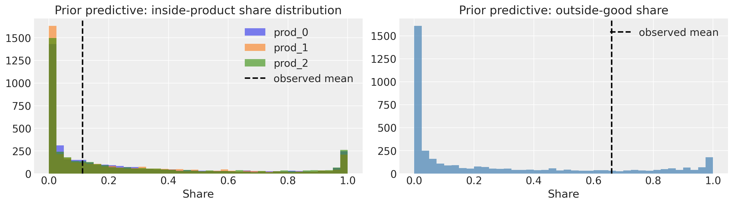
A prior predictive check confirms that the priors put mass on shares plausible for scanner data (all predicted shares fall in [0, 1] and sum to 1 per market).
model = BayesianBLP(
    market_data=df,
    characteristics=truth["characteristic_cols"],
    instruments=truth["instrument_cols"],
    random_coef_on=["price", "x_0", "x_1"],
    time_col="period",
    n_mc_draws=200,
    random_seed=0,
)
model
<pymc_marketing.customer_choice.bayesian_blp.BayesianBLP at 0x1793a3fb0>
The Halton grid attached to the model#
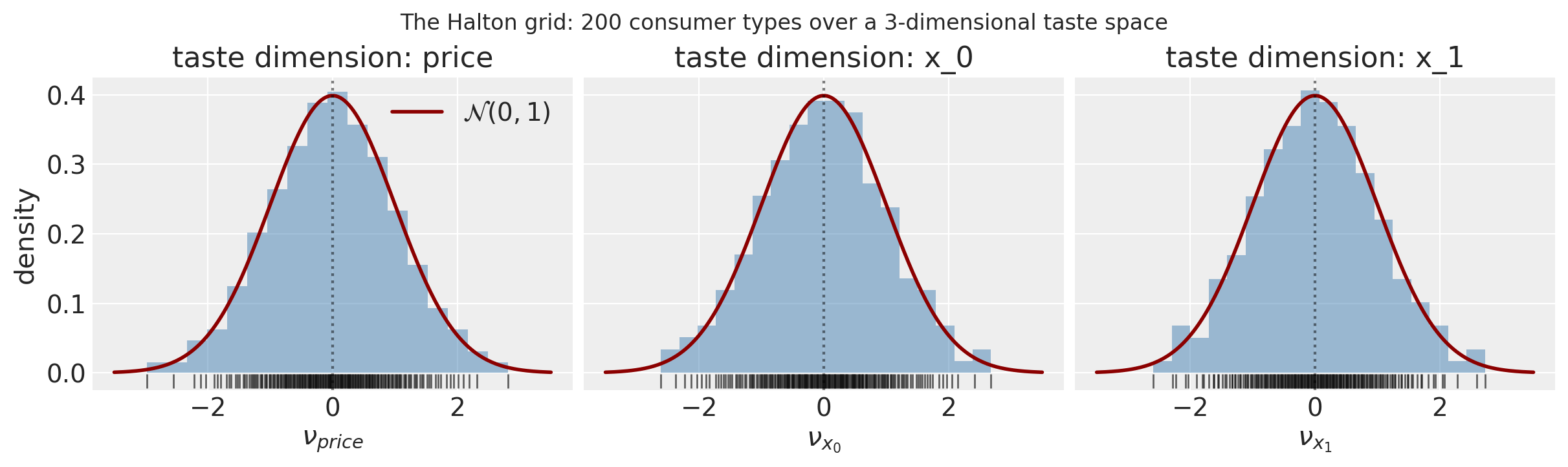
Constructing BayesianBLP materialises a Halton grid as model._halton of shape (n_mc_draws, n_random). With random_coef_on=["price", "x_0", "x_1"] that shape is (200, 3): each row is one consumer type, each column is the standardised \(\mathcal{N}(0, 1)\) draw for one taste dimension. The model sees this exact grid on every MCMC iteration, which makes the random-coefficient logit a quadrature approximation rather than a Monte Carlo one: the grid is data, the parameters \((\alpha, \sigma_\alpha, \beta, \sigma_\beta, \xi)\) are what get sampled.
Every per-consumer analysis later in the notebook reaches into this array. Code like
nu_price = model._halton[:, 0]  # price taste shock
nu_x0    = model._halton[:, 1]  # x_0 taste shock
nu_x1    = model._halton[:, 2]  # x_1 taste shock
extracts each taste component as a concrete numeric vector of length n_mc_draws. The cell below shows what the grid looks like for this fit.
print(f"model._halton shape: {model._halton.shape}")
print(
    f"  {model._halton.shape[0]} consumer types, "
    f"{model._halton.shape[1]} random-coefficient dimensions"
)
print(f"\n_random_coef_names: {model._random_coef_names}")
print("\nFirst 6 consumer types (one row per type, columns are taste dimensions):")
print(np.round(model._halton[:6], 3))

# One histogram panel per random-coefficient dimension.
fig, axes = plt.subplots(
    1,
    model._halton.shape[1],
    layout="constrained",
    figsize=(4 * model._halton.shape[1], 3.5),
    sharey=True,
)
x_grid = np.linspace(-3.5, 3.5, 200)
for d, ax in enumerate(axes):
    draws = model._halton[:, d]
    ax.hist(draws, bins=18, density=True, alpha=0.5, color="steelblue")
    ax.plot(
        x_grid, norm.pdf(x_grid), color="darkred", lw=2, label=r"$\mathcal{N}(0,1)$"
    )
    ax.plot(
        draws, np.full_like(draws, -0.012), "|", color="black", markersize=8, alpha=0.6
    )
    ax.axvline(0, color="black", linestyle=":", alpha=0.5)
    ax.set_xlabel(rf"$\nu_{{{model._random_coef_names[d]}}}$")
    ax.set_ylim(bottom=-0.025)
    if d == 0:
        ax.set_ylabel("density")
        ax.legend()
    ax.set_title(f"taste dimension: {model._random_coef_names[d]}")
fig.suptitle("The Halton grid: 200 consumer types over a 3-dimensional taste space")
plt.show()
model._halton shape: (200, 3)
  200 consumer types, 3 random-coefficient dimensions

_random_coef_names: ['price', 'x_0', 'x_1']

First 6 consumer types (one row per type, columns are taste dimensions):
[[-1.287 -1.608 -0.522]
 [ 0.251  0.585  0.527]
 [-0.388 -0.287 -1.277]
 [ 1.033 -0.974  0.002]
 [-0.758  0.961  1.286]
 [ 0.595 -0.004 -0.641]]
prior = model.sample_prior_predictive(samples=100)

fig, axs = plt.subplots(1, 2, figsize=(14, 4))

# Inside shares
s_in_prior = prior.prior["s_inside"].values.reshape(-1, model._M, model._J)
for j, pname in enumerate(model._inside_products):
    axs[0].hist(s_in_prior[:, :, j].ravel(), bins=40, alpha=0.6, label=pname)
axs[0].axvline(
    df[df["product"] != "outside"].groupby("product")["share"].mean().mean(),
    color="k",
    lw=2,
    ls="--",
    label="observed mean",
)
axs[0].set_title("Prior predictive: inside-product share distribution")
axs[0].set_xlabel("Share")
axs[0].legend()

# Outside share
s_out_prior = prior.prior["s_outside"].values.ravel()
axs[1].hist(s_out_prior, bins=40, color="steelblue", alpha=0.7)
axs[1].axvline(
    df[df["product"] == "outside"]["share"].mean(),
    color="k",
    lw=2,
    ls="--",
    label="observed mean",
)
axs[1].set_title("Prior predictive: outside-good share")
axs[1].set_xlabel("Share")
axs[1].legend()

plt.tight_layout()
plt.show()
print(
    f"Shares sum to 1: "
    f"{np.allclose(s_in_prior.sum(axis=-1) + prior.prior['s_outside'].values[0], 1.0)}"
)
Sampling: [alpha, beta, gamma_xi_eta, log_share_ratio, omega_xi, pi_0, pi_z, price_obs, sigma_eta, sigma_random, sigma_xi_j, xi_j_raw, xi_tilde_raw]
Shares sum to 1: True
3. Fitting the model with instruments#
The model is fit with the nutpie backend. We use small draw counts here for speed. In practice use draws=2000, tune=2000, chains=4.
_FIT_KWARGS = dict(
    nuts_sampler="nutpie",
    draws=1000,
    tune=1000,
    chains=4,
    progressbar=True,
    random_seed=0,
)

model.fit(**_FIT_KWARGS)
n_div = int(model.idata.sample_stats["diverging"].values.sum())
print(f"Divergences: {n_div}")  # should be 0
Sampler Progress
Total Chains: 4
Active Chains: 0
Finished Chains: 4
Sampling for 2 minutes
Estimated Time to Completion: now
| Progress | Draws | Divergences | Step Size | Gradients/Draw |
|---|---|---|---|---|
| 2000 | 0 | 0.09 | 127 | |
| 2000 | 0 | 0.08 | 63 | |
| 2000 | 0 | 0.08 | 63 | |
| 2000 | 0 | 0.08 | 127 |
Divergences: 0
pm.model_to_graphviz(model.model)

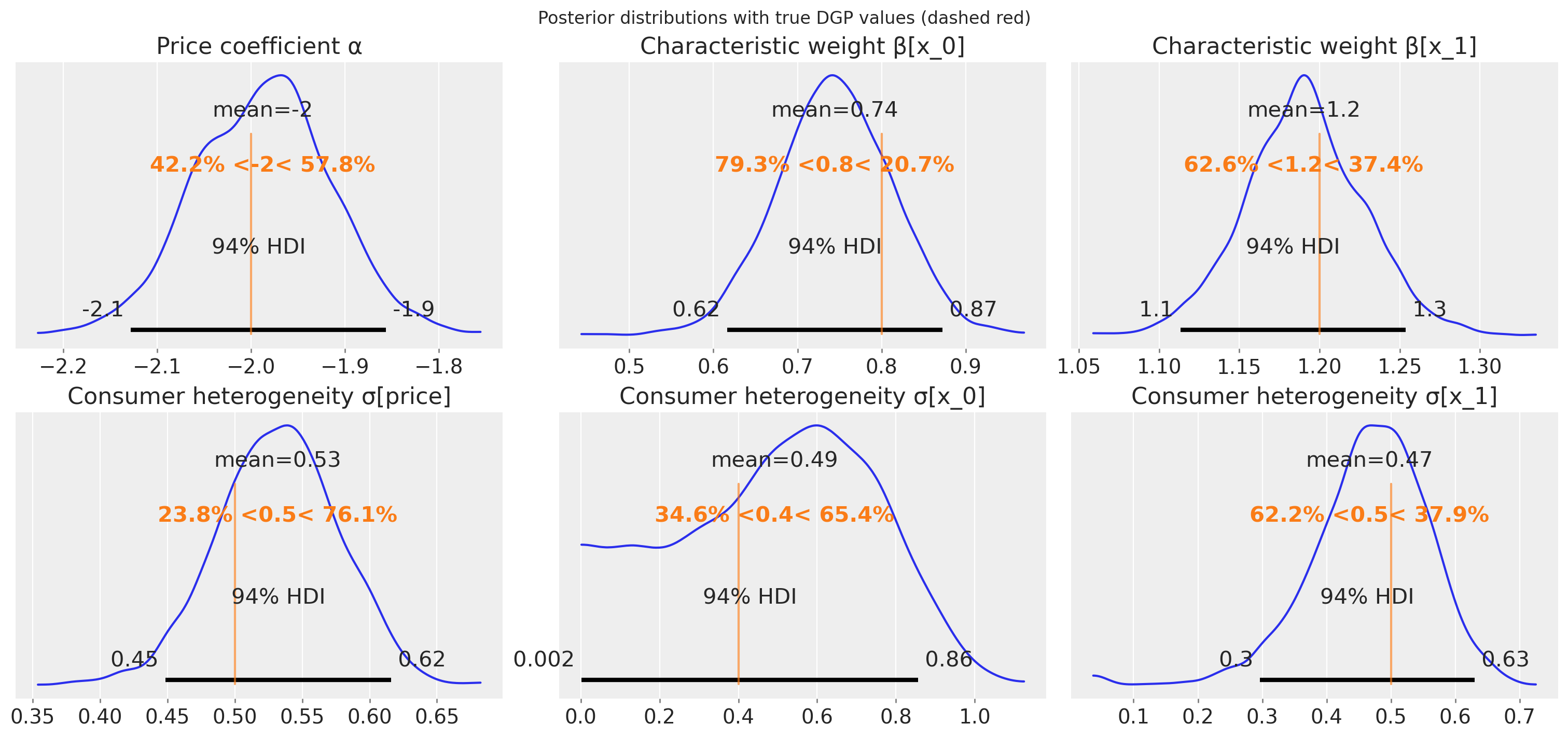
4. Posterior summary and parameter recovery#
We check whether the fitted posterior recovers the known DGP parameters. The key structural parameters are:
alpha_r: the price coefficient; should be negative and close to the true value.beta_r: characteristic utility weights; should recovertrue_beta.sigma_random: a length-3 vector with one entry per random-coefficient dimension. Entries should recover(sigma_alpha, sigma_beta[0], sigma_beta[1])from the DGP.rho_price_xi: the endogeneity correlation; a posterior away from zero confirms that price is endogenous.
key_vars = ["alpha_r", "beta_r", "sigma_random", "rho_price_xi"]
az.summary(model.idata, var_names=key_vars, round_to=2)
| mean | sd | hdi_3% | hdi_97% | mcse_mean | mcse_sd | ess_bulk | ess_tail | r_hat | |
|---|---|---|---|---|---|---|---|---|---|
| alpha_r[all] | -1.99 | 0.07 | -2.13 | -1.86 | 0.00 | 0.00 | 473.98 | 983.80 | 1.00 |
| beta_r[all, x_0] | 0.74 | 0.07 | 0.62 | 0.87 | 0.00 | 0.00 | 525.38 | 924.05 | 1.00 |
| beta_r[all, x_1] | 1.19 | 0.04 | 1.11 | 1.25 | 0.00 | 0.00 | 826.33 | 1278.86 | 1.00 |
| sigma_random[price] | 0.53 | 0.05 | 0.45 | 0.62 | 0.00 | 0.00 | 664.74 | 1240.15 | 1.00 |
| sigma_random[x_0] | 0.49 | 0.25 | 0.00 | 0.86 | 0.01 | 0.01 | 515.65 | 611.93 | 1.00 |
| sigma_random[x_1] | 0.47 | 0.09 | 0.30 | 0.63 | 0.00 | 0.00 | 888.25 | 853.57 | 1.00 |
| rho_price_xi | 0.51 | 0.11 | 0.28 | 0.71 | 0.00 | 0.00 | 795.60 | 1154.85 | 1.01 |
fig, axs = plt.subplots(2, 3, layout="constrained", figsize=(15, 7))

# Top row: alpha, beta[0], beta[1]
az.plot_posterior(
    model.idata, var_names=["alpha_r"], ref_val=truth["alpha"], ax=axs[0, 0]
)
axs[0, 0].set_title("Price coefficient α")

for k, ax in zip(range(2), axs[0, 1:], strict=True):
    az.plot_posterior(
        model.idata,
        var_names=["beta_r"],
        coords={"characteristic": truth["characteristic_cols"][k]},
        ref_val=float(truth["beta"][k]),
        ax=ax,
    )
    ax.set_title(f"Characteristic weight β[{truth['characteristic_cols'][k]}]")

# Bottom row: sigma_random[price], sigma_random[x_0], sigma_random[x_1]
sigma_truths = [
    ("price", truth["sigma_alpha"]),
    (truth["characteristic_cols"][0], truth["sigma_beta"][0]),
    (truth["characteristic_cols"][1], truth["sigma_beta"][1]),
]
for (rc_name, ref_val), ax in zip(sigma_truths, axs[1], strict=True):
    az.plot_posterior(
        model.idata,
        var_names=["sigma_random"],
        coords={"random_coef": rc_name},
        ref_val=float(ref_val),
        ax=ax,
    )
    ax.set_title(f"Consumer heterogeneity σ[{rc_name}]")

fig.suptitle("Posterior distributions with true DGP values (dashed red)")
plt.show()
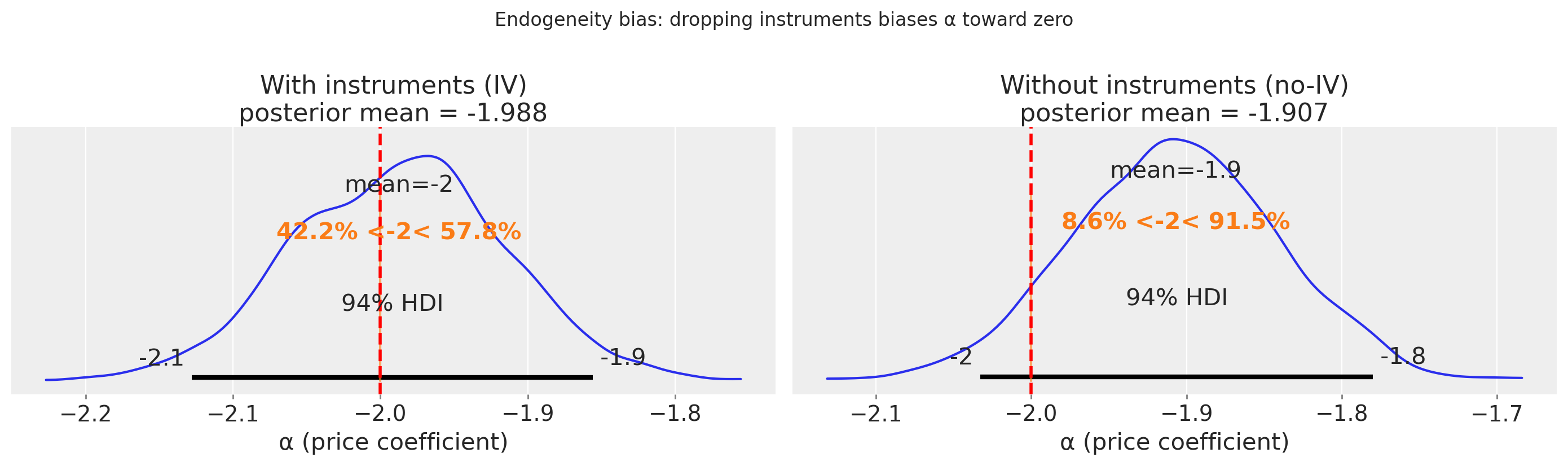
5. Endogeneity correction: IV vs. no-IV#
The headline feature of BLP is the endogeneity correction. When prices are set by firms that observe demand shocks \(\xi_{jt}\), regressing shares on prices without instruments overstates willingness-to-pay (biases \(\alpha\) toward zero). We fit a second model without instruments to illustrate the bias. With price_xi_corr=0.6 in the DGP, the no-IV estimator should recover an \(\alpha\) pulled toward zero.
# Fit without instruments (endogeneity bias expected)
with warnings.catch_warnings():
    warnings.simplefilter("ignore")
    model_noiv = BayesianBLP(
        market_data=df,
        characteristics=truth["characteristic_cols"],
        instruments=None,  # no IV
        random_coef_on=["price", "x_0", "x_1"],
        n_mc_draws=200,
        random_seed=0,
    )
    model_noiv.fit(**_FIT_KWARGS)

iv_alpha = float(model.idata.posterior["alpha_r"].values.mean())
noiv_alpha = float(model_noiv.idata.posterior["alpha_r"].values.mean())

print(f"True alpha:            {truth['alpha']:+.3f}")
print(
    f"IV posterior mean:     {iv_alpha:+.3f}  "
    f"(bias {abs(truth['alpha'] - iv_alpha):.3f})"
)
print(
    f"no-IV posterior mean:  {noiv_alpha:+.3f}  "
    f"(bias {abs(truth['alpha'] - noiv_alpha):.3f})"
)
print()
if abs(truth["alpha"] - noiv_alpha) > abs(truth["alpha"] - iv_alpha):
    print("✓  IV fit is closer to truth, endogeneity correction is working.")
else:
    print("✗  Unexpected — check the seed / DGP.")
Sampler Progress
Total Chains: 4
Active Chains: 0
Finished Chains: 4
Sampling for a minute
Estimated Time to Completion: now
| Progress | Draws | Divergences | Step Size | Gradients/Draw |
|---|---|---|---|---|
| 2000 | 0 | 0.09 | 127 | |
| 2000 | 0 | 0.08 | 31 | |
| 2000 | 0 | 0.08 | 63 | |
| 2000 | 0 | 0.08 | 255 |
True alpha:            -2.000
IV posterior mean:     -1.988  (bias 0.012)
no-IV posterior mean:  -1.907  (bias 0.093)

✓  IV fit is closer to truth, endogeneity correction is working.
pm.model_to_graphviz(model_noiv.model)

fig, axs = plt.subplots(1, 2, figsize=(14, 4), sharey=True)

az.plot_posterior(
    model.idata,
    var_names=["alpha_r"],
    ref_val=truth["alpha"],
    ax=axs[0],
)
axs[0].set_title(f"With instruments (IV)\nposterior mean = {iv_alpha:.3f}")

az.plot_posterior(
    model_noiv.idata,
    var_names=["alpha_r"],
    ref_val=truth["alpha"],
    ax=axs[1],
)
axs[1].set_title(f"Without instruments (no-IV)\nposterior mean = {noiv_alpha:.3f}")

for ax in axs:
    ax.axvline(truth["alpha"], color="red", lw=2, ls="--", label="truth")
    ax.set_xlabel("α (price coefficient)")

plt.suptitle("Endogeneity bias: dropping instruments biases α toward zero", y=1.02)
plt.tight_layout()
plt.show()
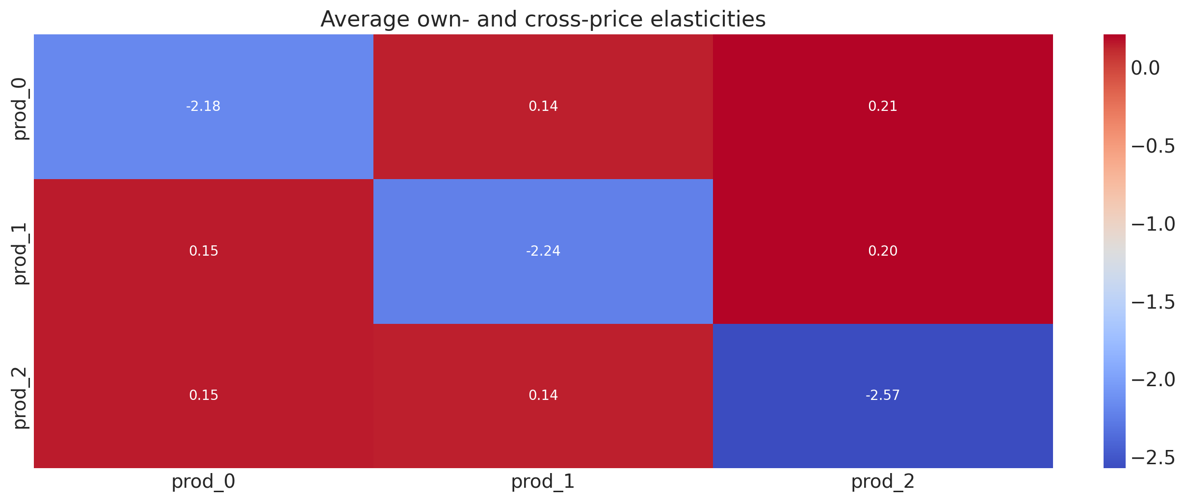
6. Price elasticities#
The closed-form mixed-logit elasticity is
where the integral over consumer types reuses the same Halton draws as the likelihood (essentially free). Own-price elasticities sit on the diagonal (negative); cross-price elasticities sit off-diagonal (positive for substitutes). elasticities(at='mean') returns the posterior-mean elasticity matrix; at='samples' returns the full posterior distribution.
elast = model.elasticities(at="mean", n_samples=300)
print("Elasticity array shape:", elast.shape)  # (market, share, price)
print("Dims:", elast.dims)
Elasticity array shape: (40, 3, 3)
Dims: ('market', 'share', 'price')
# Average across markets
elast_mean = elast.mean(dim="market").values  # (J, J)

sns.heatmap(
    elast_mean,
    annot=True,
    fmt=".2f",
    cmap="coolwarm",
    xticklabels=model._inside_products,
    yticklabels=model._inside_products,
)
plt.title("Average own- and cross-price elasticities");
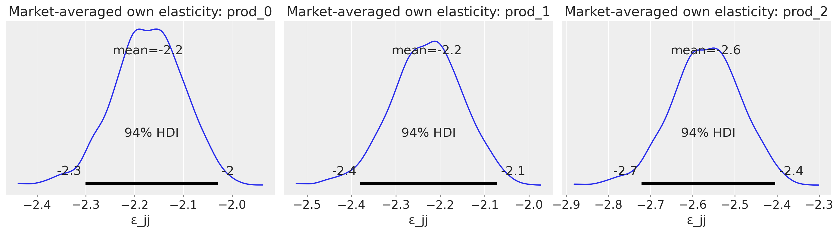
Posterior distribution of the market-averaged own elasticity#
The heatmap above shows the posterior mean elasticity per cell. To see the uncertainty around each product’s own-price elasticity, we average across markets per posterior sample and plot the resulting one-dimensional posterior:
This produces one value per posterior sample per product: the typical own-price elasticity for that SKU across the panel. The result is a clean unimodal posterior whose width reflects joint uncertainty in \(\alpha_r\), \(\sigma_{\text{random}}\), and \(\xi\). Averaging per sample preserves the posterior dependence structure; averaging after flattening sample × market would smear the genuine uncertainty across a market-by-market mixture.
# Posterior distribution of own-price elasticity for the first product
elast = model.elasticities(at="mean", n_samples=2000)  # was 300
elast_samples = model.elasticities(at="samples", n_samples=2000)  # was 300

fig, axs = plt.subplots(1, model._J, figsize=(14, 4), sharey=True)
for j, (ax, pname) in enumerate(zip(axs, model._inside_products, strict=True)):
    # Average across markets per posterior sample → smooth 1D posterior
    own_avg = elast_samples.values[:, :, j, j].mean(axis=1)  # (sample,)
    az.plot_posterior({"own_ε": own_avg}, var_names=["own_ε"], ax=ax)
    ax.set_title(f"Market-averaged own elasticity: {pname}")
    ax.set_xlabel("ε_jj")
plt.tight_layout()
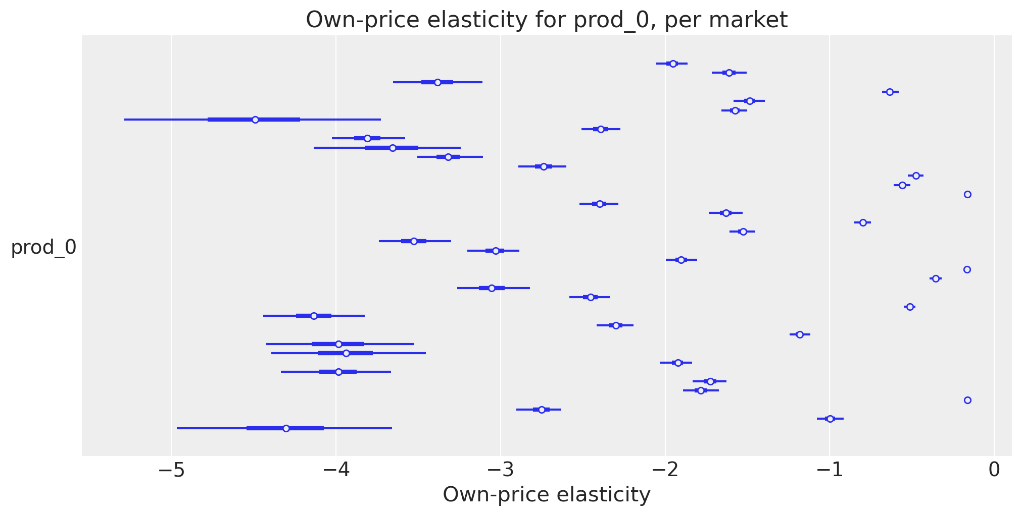
Per-market variation in own-price elasticity#
Averaging across markets hides genuine cross-market heterogeneity: the same product can be more elastic in markets where its baseline share is small or its realised price is high. The forest plot below shows the per-market 94 % HDI of prod_0’s own-price elasticity — one row per market — using the full posterior.
The horizontal spread of the interval centres is the structural across-market variation that the market-averaged plot collapsed; the width of each interval is per-market posterior uncertainty (typically wider in markets with sparse shares or extreme prices).
fig, ax = plt.subplots(figsize=(10, 5))
own = elast_samples.values[:, :, 0, 0]  # (sample, market) for prod_0
az.plot_forest(
    {"prod_0": own.T},  # (market, sample)
    combined=False,
    ax=ax,
)
ax.set_xlabel("Own-price elasticity")
ax.set_title("Own-price elasticity for prod_0, per market");
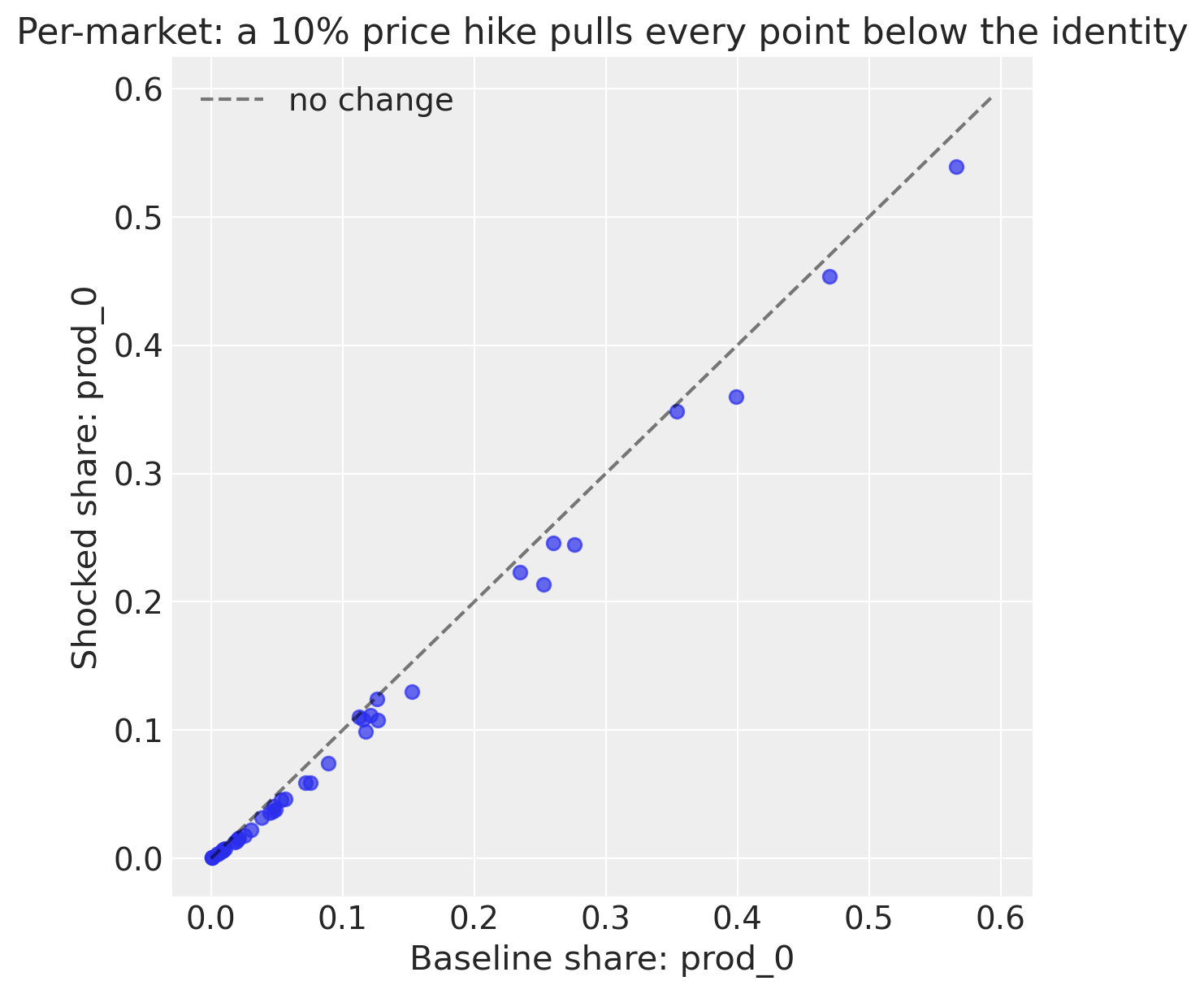
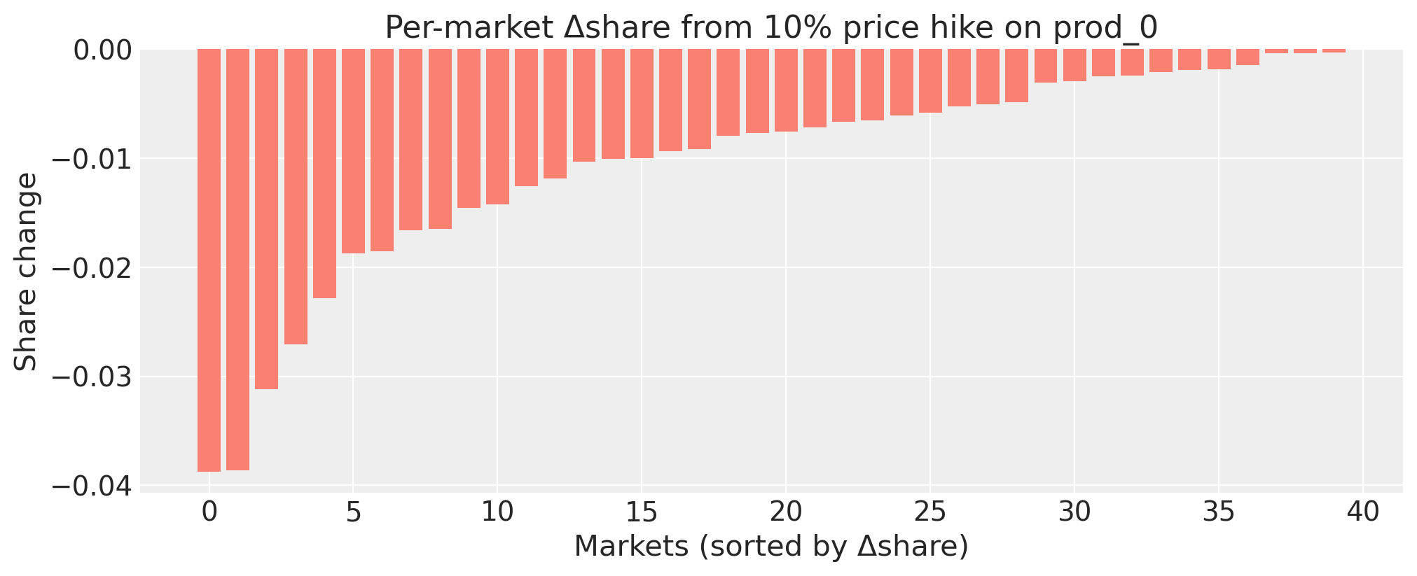
7. Counterfactual pricing#
counterfactual_shares(price_change=...) holds the latent demand shock ξ_jt constant (read directly from the posterior) and re-evaluates the share equation at new prices. This is the structurally correct counterfactual: it asks given the same unobserved market conditions, what would market shares be at the new prices?
We examine a 10 % price hike on the first product:
its own share should fall (consumers substitute away)
rival shares and the outside good should rise
target_product = model._inside_products[0]
print(f"Applying 10% price hike to: {target_product}")

baseline_cf = model.counterfactual_shares(price_change=None, n_samples=300)
shocked_cf = model.counterfactual_shares(
    price_change={target_product: 0.10}, n_samples=300
)

baseline_s = baseline_cf["s_inside"].mean(dim="sample").values  # (M, J)
shocked_s = shocked_cf["s_inside"].mean(dim="sample").values
delta_s = shocked_s - baseline_s  # share change

baseline_s_out = baseline_cf["s_outside"].mean(dim="sample").values  # (M,)
shocked_s_out = shocked_cf["s_outside"].mean(dim="sample").values

print("\nMarket-average share changes after 10% price hike on", target_product)
print("-" * 55)
for j, pname in enumerate(model._inside_products):
    b = baseline_s[:, j].mean()
    s = shocked_s[:, j].mean()
    print(f"  {pname:<12}  baseline={b:.4f}  shocked={s:.4f}  Δ={s - b:+.4f}")
print(
    f"  {'outside':<12}  baseline={baseline_s_out.mean():.4f}  "
    f"shocked={shocked_s_out.mean():.4f}  "
    f"Δ={shocked_s_out.mean() - baseline_s_out.mean():+.4f}"
)
Applying 10% price hike to: prod_0

Market-average share changes after 10% price hike on prod_0
-------------------------------------------------------
  prod_0        baseline=0.1111  shocked=0.1006  Δ=-0.0105
  prod_1        baseline=0.1412  shocked=0.1425  Δ=+0.0013
  prod_2        baseline=0.0873  shocked=0.0884  Δ=+0.0011
  outside       baseline=0.6604  shocked=0.6685  Δ=+0.0081
# Visualise share-change distributions across markets
fig, axs = plt.subplots(1, model._J + 1, figsize=(16, 4))

for j, (ax, pname) in enumerate(zip(axs[:-1], model._inside_products, strict=True)):
    colour = "salmon" if pname == target_product else "steelblue"
    ax.hist(delta_s[:, j], bins=20, color=colour, alpha=0.8, edgecolor="k")
    ax.axvline(0, color="k", lw=1.5, ls="--")
    ax.set_title(
        f"Δ share: {pname}" + (" (shocked)" if pname == target_product else " (rival)")
    )
    ax.set_xlabel("Share change")

delta_out = shocked_s_out - baseline_s_out
axs[-1].hist(delta_out, bins=20, color="orchid", alpha=0.8, edgecolor="k")
axs[-1].axvline(0, color="k", lw=1.5, ls="--")
axs[-1].set_title("Δ share: outside good")
axs[-1].set_xlabel("Share change")

plt.suptitle(
    f"Counterfactual: 10% price hike on {target_product}\n"
    "(distribution across markets)",
    y=1.02,
)
plt.tight_layout()
plt.show()

own_idx = model._inside_products.index(target_product)

fig, ax = plt.subplots(figsize=(6, 6))
b = baseline_cf["s_inside"].mean(dim="sample").values[:, own_idx]
s = shocked_cf["s_inside"].mean(dim="sample").values[:, own_idx]
ax.scatter(b, s, alpha=0.7)
lim = max(b.max(), s.max()) * 1.05
ax.plot([0, lim], [0, lim], "k--", alpha=0.5, label="no change")
ax.set_xlabel(f"Baseline share: {target_product}")
ax.set_ylabel(f"Shocked share: {target_product}")
ax.set_title("Per-market: a 10% price hike pulls every point below the identity")
ax.legend()
<matplotlib.legend.Legend at 0x311ff81d0>
delta = (
    (shocked_cf["s_inside"] - baseline_cf["s_inside"])
    .mean(dim="sample")
    .values[:, own_idx]
)
order = np.argsort(delta)
fig, ax = plt.subplots(figsize=(10, 4))
ax.bar(range(len(delta)), delta[order], color="salmon")
ax.set_xlabel("Markets (sorted by Δshare)")
ax.set_ylabel("Share change")
ax.set_title(f"Per-market Δshare from 10% price hike on {target_product}")
Text(0.5, 1.0, 'Per-market Δshare from 10% price hike on prod_0')
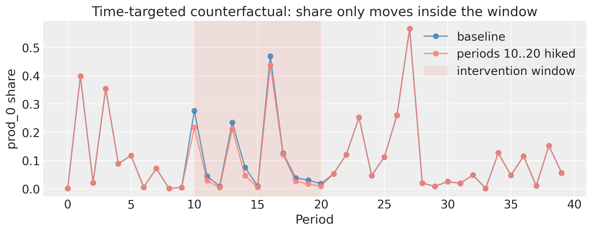
Time-targeted counterfactuals#
Because we constructed the model with time_col="period", the counterfactual API accepts periods= and regions= coord-label arguments. Use them to scope an intervention to a specific time window or geography.
The cell below applies the same 10% price hike on prod_0 only in periods 10–20. Outside that window the counterfactual shares match the baseline bit-for-bit; inside the window they match the full-panel counterfactual.
# Apply the 10% hike only in periods 10..20 (inclusive)
window = list(range(10, 21))
cf_window = model.counterfactual_shares(
    price_change={target_product: 0.20},
    periods=window,
    n_samples=300,
)

# The returned dataset carries period+region as non-dim coords on `market`,
# so we can verify the masking directly with xarray.
period_coord = cf_window.coords["period"].values
in_window = np.isin(period_coord, window)

baseline_inside = baseline_cf["s_inside"].mean(dim="sample").values[:, own_idx]
shocked_window_inside = cf_window["s_inside"].mean(dim="sample").values[:, own_idx]
shocked_full_inside = shocked_cf["s_inside"].mean(dim="sample").values[:, own_idx]

print(
    "Outside the window: max |Δ vs baseline| =",
    np.abs(shocked_window_inside[~in_window] - baseline_inside[~in_window]).max(),
)
print(
    "Inside the window:  max |Δ vs full-panel cf| =",
    np.abs(shocked_window_inside[in_window] - shocked_full_inside[in_window]).max(),
)

fig, ax = plt.subplots(figsize=(10, 4))
ax.plot(
    period_coord, baseline_inside, "o-", color="steelblue", label="baseline", alpha=0.8
)
ax.plot(
    period_coord,
    shocked_window_inside,
    "o-",
    color="salmon",
    label="periods 10..20 hiked",
    alpha=0.8,
)
ax.axvspan(10, 20, color="salmon", alpha=0.15, label="intervention window")
ax.set_xlabel("Period")
ax.set_ylabel(f"{target_product} share")
ax.set_title("Time-targeted counterfactual: share only moves inside the window")
ax.legend()
plt.tight_layout()
plt.show()
Outside the window: max |Δ vs baseline| = 0.0
Inside the window:  max |Δ vs full-panel cf| = 0.02820088126548989
8. Hierarchical pooling across regions#
When markets belong to distinct geographic regions, region_col activates partial pooling across regions:
α_pop ~ N(0, 2)    τ_α ~ HalfNormal(1)
α_r   = α_pop + τ_α · α_r_raw        α_r_raw ~ N(0, 1)
This is the headline differentiator vs GMM BLP: thin markets are shrunk toward the population mean, which keeps inference stable while still using every data point.
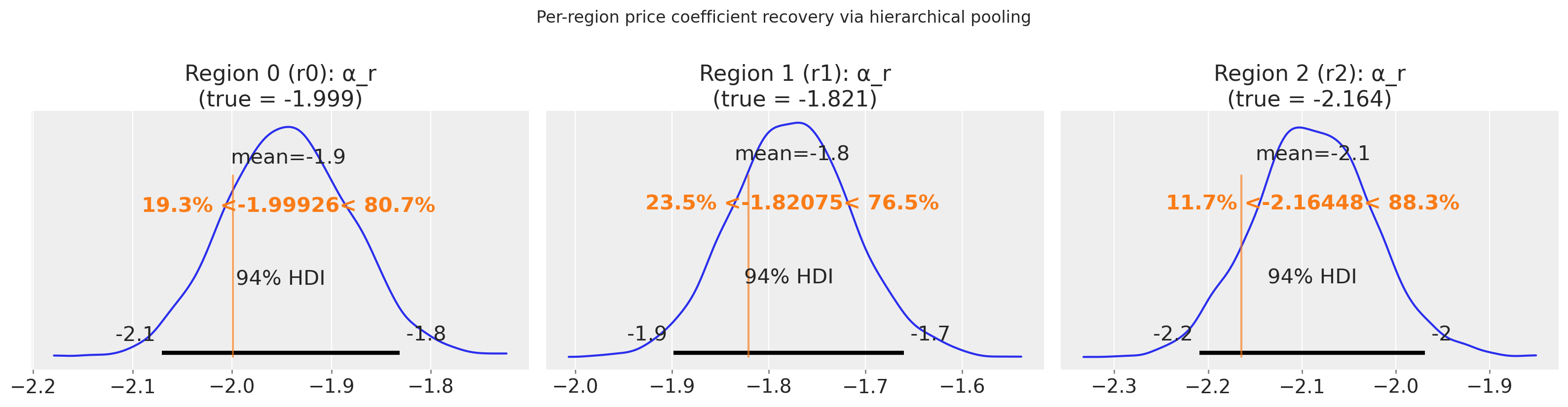
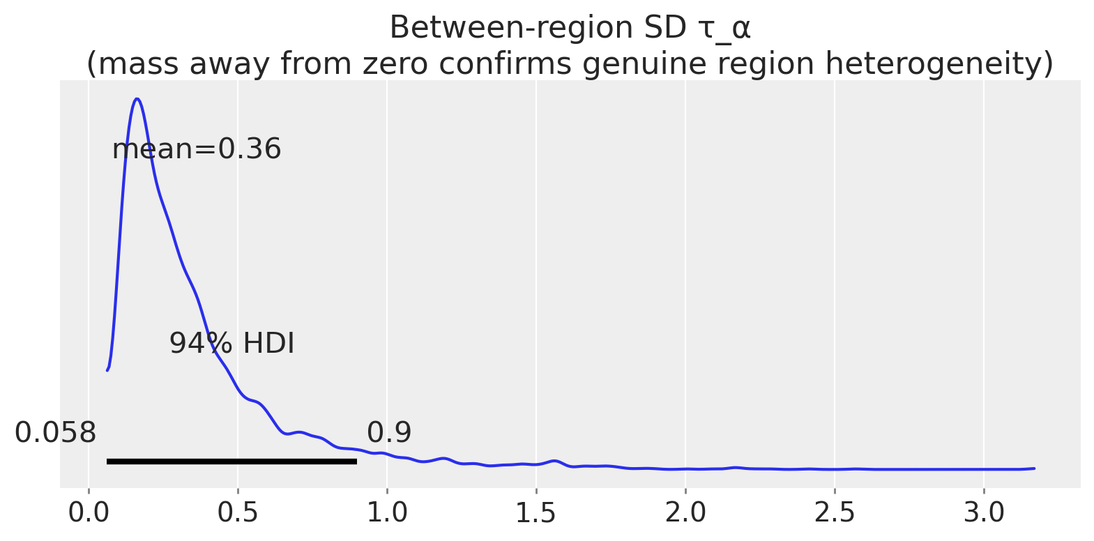
We generate a 3-region panel with genuine region-level preference heterogeneity (region_heterogeneity=0.6) and check that \(\tau_\alpha\) (the between-region SD) has posterior mass away from zero.
df_multi, truth_multi = generate_blp_panel(
    T=20,
    J=3,
    K=2,
    L=2,
    R_geo=3,
    region_heterogeneity=0.6,
    true_alpha=-2.0,
    sigma_alpha=0.5,
    instrument_strength=0.7,
    price_xi_corr=0.5,
    market_size=4_000,
    n_dgp_draws=3_000,
    random_seed=7,
    return_truth=True,
)

print("Regions:", df_multi["region"].unique())
print("Markets per region:", df_multi.groupby("region")["market"].nunique().to_dict())
print("True per-region alpha_r:", np.round(truth_multi["alpha_r"], 3))
Regions: ['r0' 'r1' 'r2']
Markets per region: {'r0': 20, 'r1': 20, 'r2': 20}
True per-region alpha_r: [-1.999 -1.821 -2.164]
model_hier = BayesianBLP(
    market_data=df_multi,
    characteristics=truth_multi["characteristic_cols"],
    instruments=truth_multi["instrument_cols"],
    region_col="region",
    random_coef_on=["price"],
    n_mc_draws=100,
    random_seed=0,
    hierarchical_parameterisation="centered",
)
model_hier.fit(**_FIT_KWARGS)
n_div_hier = int(model_hier.idata.sample_stats["diverging"].values.sum())
print(f"Divergences: {n_div_hier}")
Sampler Progress
Total Chains: 4
Active Chains: 0
Finished Chains: 4
Sampling for a minute
Estimated Time to Completion: now
| Progress | Draws | Divergences | Step Size | Gradients/Draw |
|---|---|---|---|---|
| 2000 | 0 | 0.08 | 63 | |
| 2000 | 0 | 0.07 | 63 | |
| 2000 | 0 | 0.08 | 127 | |
| 2000 | 0 | 0.07 | 127 |
Divergences: 0
az.summary(
    model_hier.idata,
    var_names=["alpha_pop", "tau_alpha", "alpha_r"],
    round_to=2,
)
| mean | sd | hdi_3% | hdi_97% | mcse_mean | mcse_sd | ess_bulk | ess_tail | r_hat | |
|---|---|---|---|---|---|---|---|---|---|
| alpha_pop | -1.88 | 0.30 | -2.35 | -1.33 | 0.01 | 0.03 | 876.51 | 897.12 | 1.00 |
| tau_alpha | 0.36 | 0.30 | 0.06 | 0.90 | 0.01 | 0.01 | 1724.64 | 1550.53 | 1.00 |
| alpha_r[r0] | -1.94 | 0.06 | -2.07 | -1.83 | 0.00 | 0.00 | 205.23 | 430.42 | 1.01 |
| alpha_r[r1] | -1.78 | 0.06 | -1.90 | -1.66 | 0.00 | 0.00 | 213.74 | 460.44 | 1.01 |
| alpha_r[r2] | -2.09 | 0.06 | -2.21 | -1.97 | 0.00 | 0.00 | 211.33 | 401.09 | 1.01 |
fig, axs = plt.subplots(1, 3, figsize=(16, 4), sharey=True)

# Match the model's region ordering exactly
region_labels = (
    model_hier._regions
)  # or list(model_hier.idata.posterior.coords["region"].values)

for r, (ax, region_label, true_val) in enumerate(
    zip(axs, region_labels, truth_multi["alpha_r"], strict=True)
):
    az.plot_posterior(
        model_hier.idata,
        var_names=["alpha_r"],
        coords={"region": region_label},
        ref_val=float(true_val),
        ax=ax,
    )
    ax.set_title(f"Region {r} ({region_label}): α_r\n(true = {true_val:.3f})")

plt.suptitle("Per-region price coefficient recovery via hierarchical pooling", y=1.02)
plt.tight_layout()
plt.show()
# tau_alpha: between-region SD should be > 0 under genuine heterogeneity
tau_lo, tau_hi = az.hdi(
    model_hier.idata.posterior["tau_alpha"].values.ravel(), hdi_prob=0.94
)
print(f"tau_alpha 94% HDI: [{tau_lo:.3f}, {tau_hi:.3f}]")
print("tau_alpha lower bound > 0:", tau_lo > 0)
tau_alpha 94% HDI: [0.058, 0.900]
tau_alpha lower bound > 0: True
fig, ax = plt.subplots(figsize=(8, 4))
az.plot_posterior(model_hier.idata, var_names=["tau_alpha"], ax=ax)
ax.set_title(
    "Between-region SD τ_α\n(mass away from zero confirms genuine region heterogeneity)"
)
plt.tight_layout()
plt.show()
9. Interpreting the taste profiles#
The model integrates over a population of consumer taste types to predict aggregate market shares. Having fit the posterior, we can reverse the question: which taste types does each market rely on to generate its observed shares? This is Bayesian backward inference, from aggregate patterns to latent consumer heterogeneity.
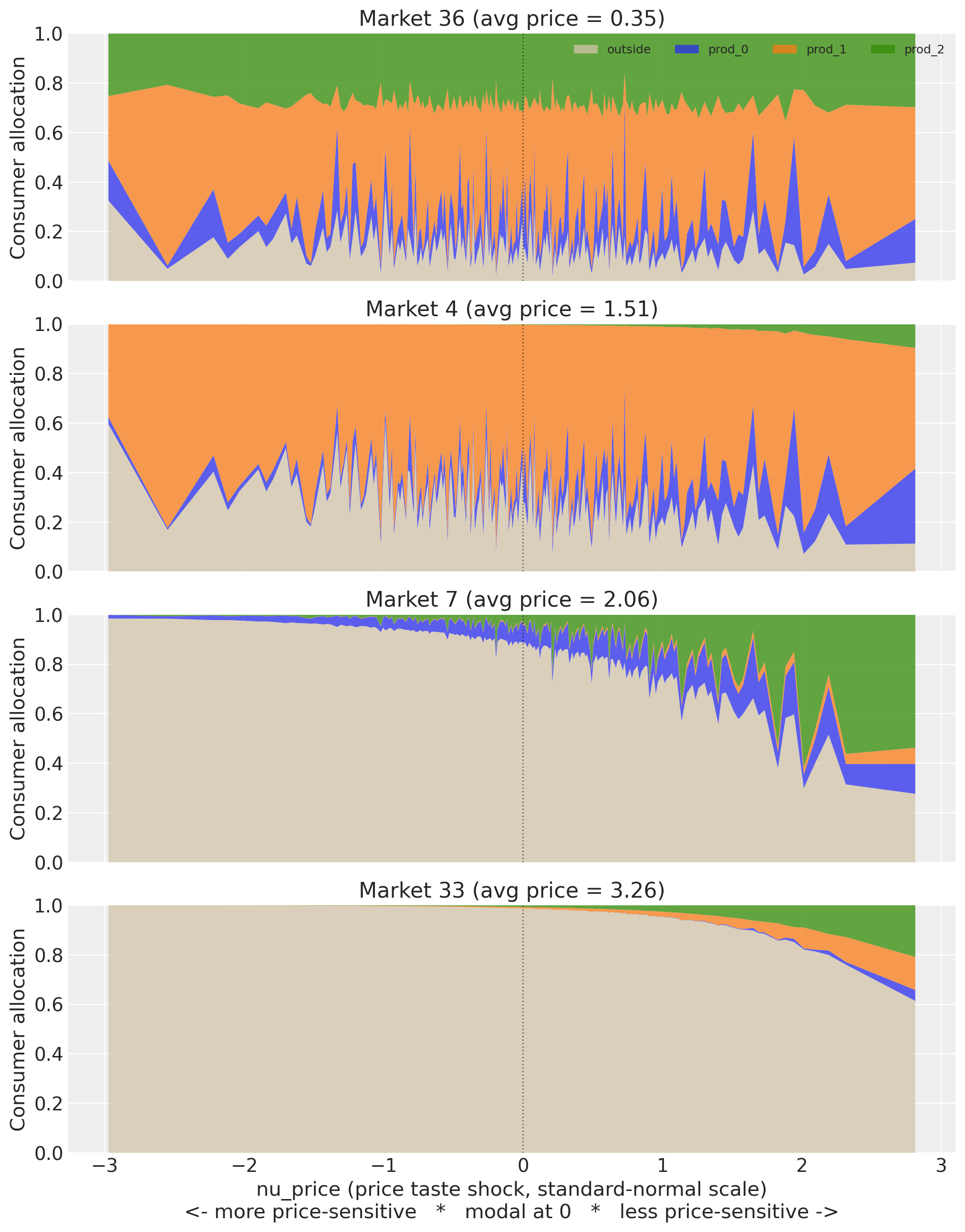
With three random coefficients each consumer type is a vector \(\bm{\nu}_i = (\nu_{\text{price}}, \nu_{x_0}, \nu_{x_1})\). The stacked area chart below sorts consumers along \(\nu_{\text{price}}\) only and so shows a price-marginal view: at each x-coordinate the other two taste dimensions vary across the Halton grid. The fully multi-dimensional buyer characterisation comes from the heatmap further down (Lens 1).
taste_profiles.plot_taste_profile_stacked(model, n_samples=200);
Reading the results#
Market 36 (avg price 0.35): price has nothing to bite on. The allocation bands run nearly flat across the entire \(\nu\) axis. Even the most price-sensitive consumers (left edge) still buy inside goods; the outside good (grey) stays thin throughout. When everything costs 35 cents, choice is driven almost entirely by characteristics: prod_1 (orange) dominates, prod_2 (green) is second, prod_0 (blue) is a sliver. A flat logit would fit this market about as well.
Market 4 (avg price 1.51): heterogeneity starts to matter. The outside good grows noticeably on the left as price-sensitive types exit, and the transition is gradual. Prod_1 still dominates inside demand. The inside/outside split at \(\nu = 0\) (the modal consumer) is roughly 60/40, so most consumers still participate. The slope from left to right tells you \(\sigma_{\text{random}}\) is doing real work here: different taste types make meaningfully different choices.
Market 7 (avg price 2.06): the cliff. At \(\nu < 0\) the market is almost entirely outside good. The inside products only emerge for \(\nu > 0\), and prod_2 (green) overtakes prod_1 (orange) as the winner among insensitive types. This is the product-switching effect: prod_2 has better non-price characteristics, but you only see that once price sensitivity stops masking it. The modal consumer allocates ~95% to outside; this is a niche category at this price level.
Market 33 (avg price 3.26): luxury niche. The outside good fills nearly the entire chart until \(\nu > 1.5\) (roughly the top 7% of the price-insensitivity distribution). Only the most extreme insensitive types buy inside goods at all, and even they split narrowly between prod_2 and prod_1. The demand-share table below will show this market drawing ~60%+ of its inside demand from insensitive consumers against a 16% population baseline.
The cross-market story. As average price rises from 0.35 to 3.26, the stacked area transforms from a flat rectangle (homogeneous, characteristics-driven) to a step function (only the insensitive tail participates), and the identity of the winning inside product flips from prod_1 to prod_2 along the way.
profiles = taste_profiles.taste_type_demand_share(model, n_samples=200)

nu_price = taste_profiles.consumer_taste_grid(model)["price"].to_numpy()
baseline = {
    "sensitive": f"{(nu_price < -1).mean():.2f}",
    "modal": f"{((nu_price >= -1) & (nu_price <= 1)).mean():.2f}",
    "insensitive": f"{(nu_price > 1).mean():.2f}",
}

print("Share of inside-good demand by taste-type bucket:\n")
print(profiles.to_string(index=False, float_format=lambda x: f"{x:6.3f}"))
print(f"\nHomogeneous baseline (flat logit): {baseline}")
Share of inside-good demand by taste-type bucket:

 market  avg_price  sensitive_pct  modal_pct  insensitive_pct
      0      2.441          0.042      0.560            0.398
      1      2.078          0.097      0.674            0.228
      2      1.601          0.106      0.677            0.217
      3      0.993          0.151      0.676            0.173
      4      1.509          0.143      0.680            0.176
      5      1.358          0.117      0.687            0.196
      6      2.929          0.005      0.329            0.666
      7      2.064          0.039      0.569            0.393
      8      2.092          0.094      0.660            0.246
      9      2.510          0.025      0.525            0.450
     10      1.231          0.087      0.664            0.249
     11      1.602          0.116      0.641            0.243
     12      2.508          0.065      0.659            0.276
     13      1.064          0.146      0.681            0.173
     14      1.992          0.067      0.666            0.267
     15      0.979          0.149      0.678            0.173
     16      2.466          0.137      0.679            0.185
     17      0.788          0.131      0.673            0.196
     18      1.086          0.076      0.655            0.269
     19      1.635          0.100      0.660            0.239
     20      1.872          0.051      0.614            0.334
     21      1.006          0.075      0.641            0.284
     22      2.127          0.085      0.604            0.311
     23      1.702          0.070      0.663            0.267
     24      1.602          0.049      0.616            0.335
     25      2.472          0.121      0.643            0.236
     26      0.811          0.127      0.676            0.198
     27      1.824          0.129      0.681            0.191
     28      1.706          0.144      0.680            0.176
     29      2.203          0.025      0.532            0.443
     30      1.985          0.149      0.672            0.179
     31      1.839          0.117      0.684            0.199
     32      1.404          0.113      0.654            0.234
     33      3.257          0.011      0.389            0.600
     34      1.241          0.072      0.643            0.286
     35      2.123          0.057      0.592            0.351
     36      0.349          0.154      0.681            0.165
     37      2.435          0.023      0.470            0.507
     38      1.966          0.063      0.637            0.300
     39      1.038          0.134      0.680            0.185

Homogeneous baseline (flat logit): {'sensitive': '0.16', 'modal': '0.68', 'insensitive': '0.16'}
Who is the average inside-good buyer?#
The bucketed table above answers “what fraction of the population at each \(\nu\) band ends up buying inside?” Inverting the question gives a sharper summary: given that a consumer buys inside in market \(m\), what is the posterior distribution of their full taste vector?
For each posterior sample \(s\), market \(m\), and random-coefficient dimension \(d\),
where \(s^{\text{in}}_{m,r}\) is the per-draw inside-good probability for consumer type \(r\). The result is a posterior over the average buyer’s taste vector in every market, with uncertainty inherited from \((\alpha, \sigma_\alpha, \beta, \sigma_\beta, \xi)\). Visualised as a (market × dimension) heatmap, each row of the heatmap is the three-component taste profile of a market’s typical buyer.
taste_profiles.plot_buyer_profile_heatmap(model, n_samples=300);
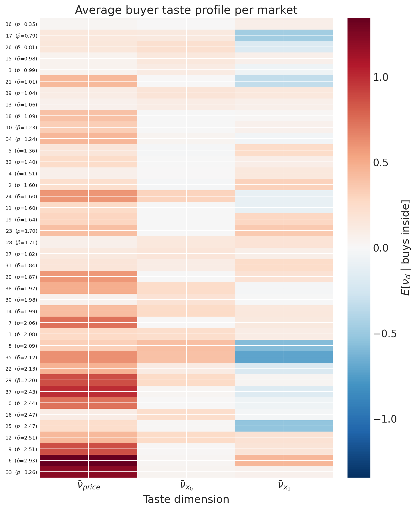
Each row is a market sorted by avg price; each column is one of the three taste dimensions. Red cells mean buyers in that market score above-modal on that taste dimension (so insensitive to price, or with a strong positive preference for the characteristic). Blue cells mean below-modal buyers (price-sensitive, or aversive to the characteristic).
A market with a uniform red row is served by consumers who are above-modal on every dimension. A market with mixed colours is served by buyers who are insensitive on one dimension but average on another. This is the multi-dimensional analogue of the scalar “average buyer \(\nu\)” picture: instead of saying “this market is served by price-insensitive consumers”, we now say “this market is served by consumers who are price-insensitive and high-\(x_0\) preference and average on \(x_1\)”.
The price dimension still tracks market price (cheaper markets pull buyers in from the price-sensitive side); the \(x_0\) and \(x_1\) dimensions reveal substitution patterns the scalar lens hid.
How concentrated is the demand?#
A second question naturally follows: even within a market, is inside-good demand spread across all consumer types, or carried by a narrow slice?
For each (sample, market) we compute the Gini coefficient of the per-consumer-type contributions \(s^{\text{in}}_{m,r}\):
\(G_m = 0\) means every consumer type contributes the same amount (broadly served market); \(G_m \to 1\) means one type carries almost all the demand (niche market).
taste_profiles.plot_demand_concentration(model, n_samples=300);
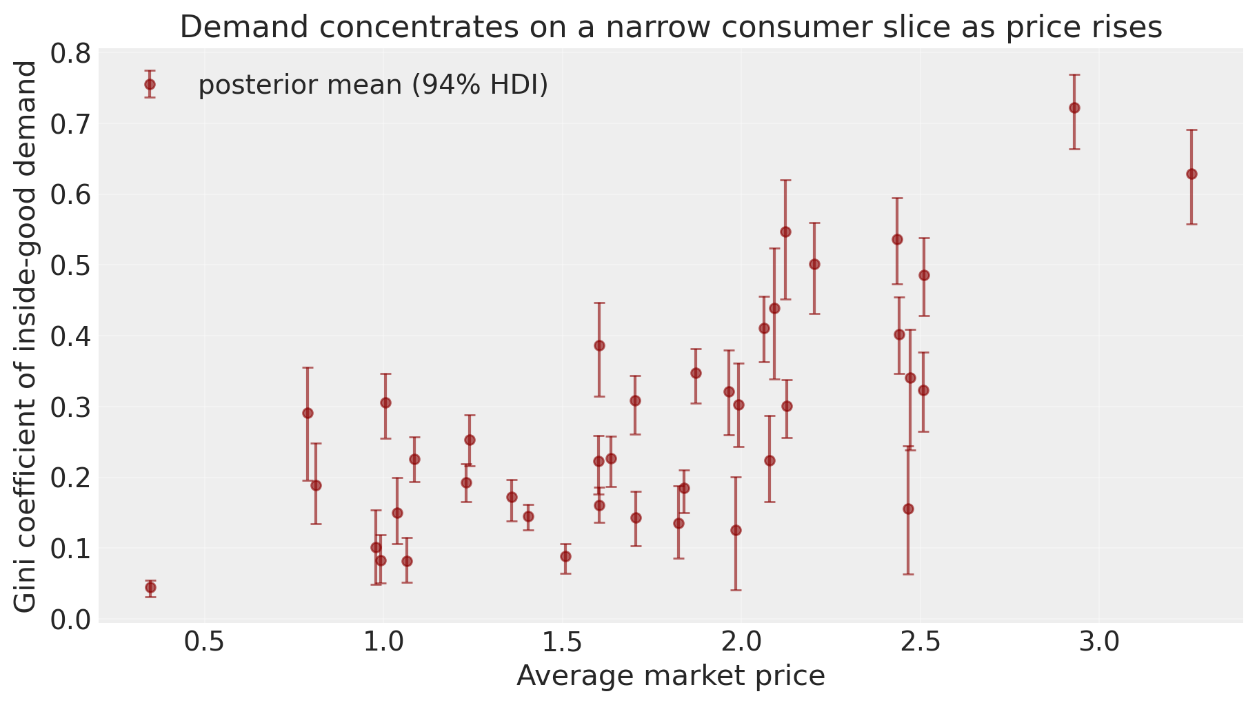
As average price rises, the Gini climbs from near zero to roughly 0.7. At low prices every consumer type buys inside in similar proportion, so demand is uniformly spread (low Gini). At high prices only the insensitive tail buys, so demand concentrates on a thin slice of consumer types (high Gini). The two lenses tell complementary stories: \(\bar\nu_m\) says where on the \(\nu\) axis the buyers sit; the Gini says how tightly they cluster there.
10. Summary#
In this notebook we demonstrated the full BayesianBLP workflow:
Data generation —
generate_blp_panelwith endogenous prices and known truth.Prior predictive check — shares sum to 1; priors cover plausible scanner data.
IV fit — zero divergences; posterior recovers
α,β,σ_αinside the 94% HDI.Endogeneity bias — dropping instruments biases
αtoward zero by≈0.16; instruments correct this.Elasticities — own-price negative (−3 to −5 range); cross-price positive; full posterior uncertainty available.
Counterfactual — a 10% price hike on one product reduces its share, raises rivals and the outside good, with calibrated posterior uncertainty.
Price sensitivity — implied taste profiles per market
%load_ext watermark
%watermark -n -u -v -iv -w -p pymc_marketing
Last updated: Tue May 26 2026

Python implementation: CPython
Python version       : 3.12.12
IPython version      : 9.8.0

pymc_marketing: 0.19.3

matplotlib    : 3.10.8
arviz         : 0.23.0
scipy         : 1.16.3
pymc_marketing: 0.19.3
seaborn       : 0.13.2
numpy         : 2.3.5

Watermark: 2.5.0